Introduction#
The PyData ecosystem has a number of core Python data containers that allow users to work with a wide array of datatypes, including:
Pandas: DataFrame, Series (columnar/tabular data)
Rapids cuDF: GPU DataFrame, Series (columnar/tabular data)
DuckDB: DuckDB is a fast in-process analytical database
Polars: Polars is a fast DataFrame library/in-memory query engine (columnar/tabular data)
Dask: DataFrame, Series (distributed/out of core arrays and columnar data)
XArray: Dataset, DataArray (labelled multidimensional arrays)
Streamz: DataFrame(s), Series(s) (streaming columnar data)
Intake: DataSource (data catalogues)
GeoPandas: GeoDataFrame (geometry data)
NetworkX: Graph (network graphs)
Many of these libraries have the concept of a high-level plotting API that lets a user generate common plot types very easily. The native plotting APIs are generally built on Matplotlib, which provides a solid foundation, but means that users miss out the benefits of modern, interactive plotting libraries for the web like Bokeh and HoloViews.
hvPlot provides a high-level plotting API built on HoloViews that provides a general and consistent API for plotting data in all the formats mentioned above.
As a first simple illustration of using hvPlot, let’s create a small set of random data in Pandas to explore:
import numpy as np
import pandas as pd

index = pd.date_range('1/1/2000', periods=1000)
df = pd.DataFrame(np.random.randn(1000, 4), index=index, columns=list('ABCD')).cumsum()

df.head()
| A | B | C | D | |
|---|---|---|---|---|
| 2000-01-01 | -0.553192 | -0.452734 | 0.867741 | -2.553237 |
| 2000-01-02 | -1.387772 | -1.037188 | 1.947172 | -2.693822 |
| 2000-01-03 | 0.475084 | 0.204218 | 1.996798 | -1.199984 |
| 2000-01-04 | 0.236249 | 1.465750 | 2.674207 | 0.848953 |
| 2000-01-05 | -0.584862 | 1.583417 | 0.782886 | 0.745620 |
Pandas default .plot()#
Pandas provides Matplotlib-based plotting by default, using the .plot() method:
%matplotlib inline

df.plot();
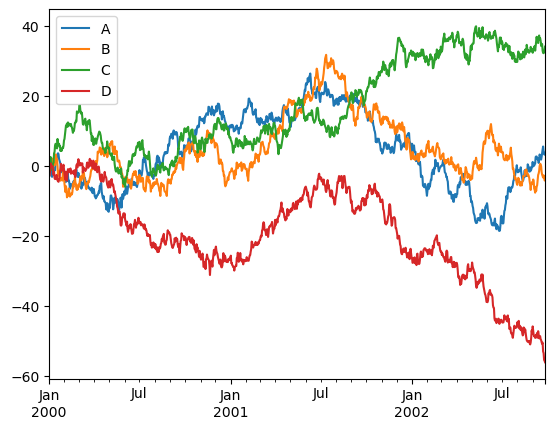
The result is a PNG image that displays easily, but is otherwise static.
Switching Pandas backend#
To allow using hvPlot directly with Pandas we have to import hvplot.pandas and swap the Pandas backend with:
import hvplot.pandas  # noqa

pd.options.plotting.backend = 'holoviews'
df.plot()
.hvplot()#
If we instead change %matplotlib inline to import hvplot.pandas and use the df.hvplot method, it will now display an interactively explorable Bokeh plot with panning, zooming, hovering, and clickable/selectable legends:
df.hvplot()
This interactive plot makes it much easier to explore the properties of the data, without having to write code to select ranges, columns, or data values manually. Note that while pandas, dask and xarray all use the .hvplot method, intake uses hvPlot as its main plotting API, which means that is available using .plot().
hvPlot native API#
For the plot above, hvPlot dynamically added the Pandas .hvplot() method, so that you can use the same syntax as with the Pandas default plotting. If you prefer to be more explicit, you can instead work directly with hvPlot objects:
from hvplot import hvPlot
hvplot.extension('bokeh')

plot = hvPlot(df)
plot(y=['A', 'B', 'C', 'D'])
Switching the plotting extension to Matplotlib or Plotly#
While the default plotting extension of hvPlot is Bokeh, it is possible to load either Matplotlib or Plotly with .extension() and later switch from a plotting library to another with .output(). More information about working with multiple plotting backends can be found in the plotting extensions guide.
hvplot.extension('matplotlib')

df.hvplot(rot=30)

Getting help#
When working inside IPython or the Jupyter notebook hvplot methods will automatically complete valid keywords, e.g. pressing tab after declaring the plot type will provide all valid keywords and the docstring:
df.hvplot.line(<TAB>
Outside an interactive environment hvplot.help will bring up information providing the kind of plot, e.g.:
hvplot.help('line')
For more detail on the available options see this page.
Working with Ruff#
In most cases, import hvplot.pandas is imported and never used directly. This will make linters like Ruff flag it as an unused-import. This can either be ignored with a # noqa: F401 or global being set in the pyproject.toml with allowed-unused-imports.
[tool.ruff.lint.pyflakes]
allowed-unused-imports = ["hvplot.pandas"]
This configuration requires Ruff version 0.6.9 or greater to be installed.
Next steps#
Now that you can see how hvPlot is used, let’s jump straight in and discover some of the more powerful things we can do with it in the Plotting section.