Using hvPlot as a Pandas user#
Prerequisites#
What? |
Why? |
|---|---|
For discovering hvPlot’s basics |
Overview#
Pandas .plot() API has slowly emerged as a de-facto standard for high-level plotting APIs in Python, providing a simple interface to generate plots directly from a DataFrame or Series object. Many libraries have implemented this interface, providing additional and varied capabilities to Python users (e.g. Plotly Express to generate Plotly plots, Xarray to generate plots from multidimensional datasets). hvPlot is one of these libraries that provides an interface heavily inspired by Pandas’, and that extends it in many ways.
Before diving more into this tutorial, let’s first list what reasons, as a Pandas user, may lead you to add hvPlot to your toolbox:
By default hvPlot uses Bokeh to generate interactive plots (zoom, pan, hover, etc.) that are very well suited for data exploration workflows, contrary to the static Matplotlib plots Pandas generates.
hvPlot doesn’t only replicate Pandas
.plotAPI but extends it in many ways, exposing many of the powerful features offered by HoloViews like handling of very large datasets (with Datashader, geographic mapping with GeoViews), automatic drill-down with widgets, easy overlay and layout, and more.hvPlot supports different objects from other data libraries (Polars, Dask, GeoPandas, Xarray, etc.), allowing you to visually explore your non-Pandas datasets with the same plotting API.
In this tutorial, we will show how to get started with hvPlot as a Pandas user, focusing on some of the basic differences between the two plotting APIs to ease your transition.
A familiar API#
As already mentioned, hvPlot’s design has been heavily inspired by Pandas’ plotting interface. This, however, doesn’t mean both APIs are fully compatible; being 100% compatible is in fact a non-goal for hvPlot. To explain why, let’s see how the two interfaces are designed.
Pandas’ plot() method is a convenient interface to Matplotlib:
        graph LR
    Pandas --> Matplotlib
On the other hand, hvPlot is a convenient interface to HoloViews, itself being an interface to plotting libraries like Bokeh, Matplotlib and Plotly:
        graph LR
    Pandas --> hvPlot
    hvPlot --> HoloViews
    HoloViews --> Bokeh
    HoloViews --> Matplotlib
    HoloViews --> Plotly
While Matplotlib and HoloViews are both visualization libraries, they are quite different in their nature, the former being a pure plotting tool (i.e. it knows how to draw pixels onto your screen) and the latter being more of a data exploration tool. These differences explain some of the differences you will observe between Pandas (more influenced by Matplotlib) and hvPlot (more influenced by HoloViews).
Yet, even if you will find some differences, as a Pandas user you should feel a great deal of familiarity when using hvPlot!
%matplotlib inline
import hvsampledata
import numpy as np
import pandas as pd

df = hvsampledata.penguins('pandas')
df.head(2)
| species | island | bill_length_mm | bill_depth_mm | flipper_length_mm | body_mass_g | sex | year | |
|---|---|---|---|---|---|---|---|---|
| 0 | Adelie | Torgersen | 39.1 | 18.7 | 181.0 | 3750.0 | male | 2007 |
| 1 | Adelie | Torgersen | 39.5 | 17.4 | 186.0 | 3800.0 | female | 2007 |
Quick way to try it out: switch Pandas backend to hvPlot#
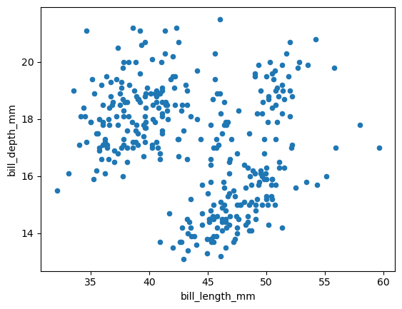
Pandas lets its users switch the plotting backend (default is Matplotlib) to a third-party library that implements the plotting interface. This means that you can keep your code as is, add one line to switch the plotting backend, and see how the plot looks like with another backend. Let’s emulate this by first generating a standard Pandas plot:
df.plot.scatter('bill_length_mm', 'bill_depth_mm');
We switch the backend to hvPlot:
pd.options.plotting.backend = 'hvplot'
From now on .plot() calls are going to leverage hvPlot to generate Bokeh plots:
df.plot.scatter('bill_length_mm', 'bill_depth_mm')
Register .hvplot() on Pandas objects#
Switching Pandas plotting backend from Matplotlib to hvPlot like we just showed is an easy way to try out hvPlot but is not the long-term approach we recommend, for two main reasons:
This possibility is only offered by Pandas that provides a special entry-point for third-party libraries to register themselves as a plotting backend, but hvPlot supports many other data libraries (Dask, Polars, GeoPandas, Xarray, etc.).
As already mentioned, Pandas’ plotting interface and hvPlot are not 100% compatible, and we find it better to be more explicit about the plotting library used.
The general mechanism to register the hvplot attribute on data objects is via a special import hvplot.<library>. Once executed, the objects of that library supported by hvPlot are equipped with the hvplot accessor. Let’s try this out with Pandas.
import hvplot.pandas # noqa
After this import, the hvplot accessor is now available on DataFrame and Series objects.
df.hvplot.scatter('bill_length_mm', 'bill_depth_mm')
df['bill_length_mm'].hvplot.hist()
pd.options.plotting.backend = 'matplotlib'
.hvplot() returns HoloViews objects#
A plot call in Pandas returns a Matplotlib Axes object. This object can be passed to Pandas’ plot API via the ax argument, for example to overlay two different plots (the ax argument is not supported in hvPlot).
plot = df.plot.scatter('bill_length_mm', 'bill_depth_mm', figsize=(4, 3))
print(plot)
Axes(0.125,0.11;0.775x0.77)
hvPlot’s plotting API returns HoloViews objects. These objects are wrappers around the original dataset, whose rich representation is a plot.
plot = df.hvplot.scatter('bill_length_mm', 'bill_depth_mm', hover_cols=['species'])
print(plot)
:Scatter [bill_length_mm] (bill_depth_mm,species)
plot
plot.data.head(2)
| species | island | bill_length_mm | bill_depth_mm | flipper_length_mm | body_mass_g | sex | year | |
|---|---|---|---|---|---|---|---|---|
| 0 | Adelie | Torgersen | 39.1 | 18.7 | 181.0 | 3750.0 | male | 2007 |
| 1 | Adelie | Torgersen | 39.5 | 17.4 | 186.0 | 3800.0 | female | 2007 |
Using HoloViews’ API, this object can be further customized.
import holoviews as hv

plot.opts(
    height=300, width=300, color=hv.dim('species'),
    cmap='Category10', show_legend=False,
).hist(['bill_length_mm','bill_depth_mm'])
Overlays and layouts#
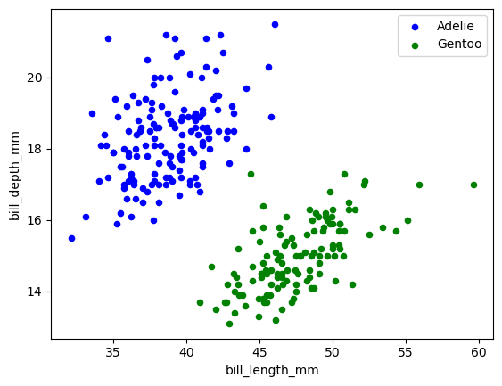
In Pandas, overlays are usually created by passing down an Axes object to another plot call via the ax argument. Layouts are created by setting subplots=True, and can be customized further with the layout argument, or with Matplotlib’s API.
The approach is quite different in hvPlot as HoloViews offers some very convenient API with * for overlaying plots and + for laying out plots. Together with the subplots argument and HoloViews’ .cols(N) method to limit the number N of plots per row, this forms an API flexible enough to handle most situations.
df1 = df.query('species == "Adelie"')
df2 = df.query('species == "Gentoo"')
ax = df1.plot.scatter('bill_length_mm', 'bill_depth_mm', color="blue", label="Adelie")
df2.plot.scatter('bill_length_mm', 'bill_depth_mm', color="green", label="Gentoo", ax=ax);
(
    df1.hvplot.scatter('bill_length_mm', 'bill_depth_mm', color="blue", label="Adelie")
    * df2.hvplot.scatter('bill_length_mm', 'bill_depth_mm', color="green", label="Gentoo")
)
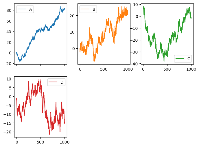
dft = pd.DataFrame(np.random.randn(1000, 4), columns=list("ABCD")).cumsum()
dft.plot.line(subplots=True, layout=(2, 3), figsize=(8, 6));
dft.hvplot.line(subplots=True, width=220).cols(3)
dft['A'].hvplot.line(width=220) + dft['B'].hvplot.line(width=220)
Setting plot dimensions#
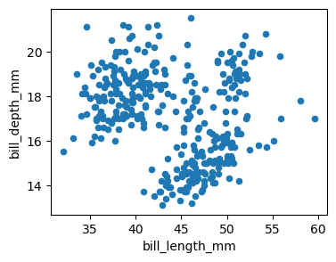
Setting plot dimensions in Pandas is done with the figsize argument that accepts a tuple (width, height) in inches. figsize is not supported in hvPlot, instead, plot dimensions are set with the width (default is 700) and height (default is 700) arguments that accept integer values in pixels.
df.plot.scatter('bill_length_mm', 'bill_depth_mm', figsize=(4, 3));
df.hvplot.scatter('bill_length_mm', 'bill_depth_mm', width=350, height=250)
Widgets-based exploration#
In the last sections we have seen some of the main differences between Pandas and hvPlot APIs, and how you could adapt your code for hvPlot’s purposes. In this section we’ll see an example of how hvPlot extends Pandas’ original API.
You can use the groupby keyword to build interactive widgets that explore different dimensions of your data. Here, we group the dataset by both 'island' and 'sex', and interactive widgets let you navigate through each combination. Click on the widgets to reveal how these factors influence the visualization of the data.
df.hvplot.scatter(x='bill_length_mm', y='bill_depth_mm', groupby=['island', 'sex'])
Saving a plot#
Saving a Bokeh plot generated with hvPlot can be done directly from your browser by clicking on the Save button in the toolbar, entering a name and pressing OK. The plot is saved as a PNG on your machine.
plot = df.hvplot.scatter('bill_length_mm', 'bill_depth_mm', width=350, height=250)
plot
Alternatively, you can save a plot using the hvplot.save() utility, passing it a plot object, a file name and optional arguments. Below, we show how to save this plot as an HTML file with all of the required resources inlined (so it can be viewed offline).
hvplot.save(plot, 'my_plot.html', resources='inline')
Matplotlib plots with hvPlot#
hvPlot can also generate Matplotlib plots.
hvplot.extension('matplotlib')
plot = df.hvplot.scatter('bill_length_mm', 'bill_depth_mm', width=350, height=250)
plot

Tip
Saving programmatically a Bokeh plot as a static file requires you to install some browser-based technology in your environment, which is doable but not the most practical approach. Instead, with the Matplotlib extension saving plots as PNG or SVG is straightforward.
hvplot.save(plot, 'my_plot.png')
hvplot.save(plot, 'my_plot.svg')
Next steps#
Visit the Pandas API compatibility reference section.
Find out more about hvPlot by exploring this website!